Scikit-Learn overview

Scikit-Learn overview#

import numpy as np
import matplotlib.pyplot as plt
from sklearn.svm import SVC
import pandas as pd

from sklearn.datasets import load_iris
from sklearn.model_selection import train_test_split
import seaborn as sns

クラス分類 (Classification)#

与えられた膨大なデータを，あらかじめ人間が割り当てたカテゴリ（クラス）に割り当てるタスク．

ここではSVM（サポートベクターマシン）のデモを行います．

擬似乱数のSEEDを設定

SEED = 42

np.random.seed(SEED)

データの読み込み

df1 = load_iris(as_frame=True)["frame"]

print("---"*10,"raw data","---"*30)
display(df1.head(10))
print("---"*10,"info","---"*30)
print(df1.info())
print("---"*10,"describe","---"*30)
print(df1.describe())

------------------------------ raw data ------------------------------------------------------------------------------------------

	sepal length (cm)	sepal width (cm)	petal length (cm)	petal width (cm)
0	5.1	3.5	1.4	0.2
1	4.9	3.0	1.4	0.2
2	4.7	3.2	1.3	0.2
3	4.6	3.1	1.5	0.2
4	5.0	3.6	1.4	0.2
5	5.4	3.9	1.7	0.4
6	4.6	3.4	1.4	0.3
7	5.0	3.4	1.5	0.2
8	4.4	2.9	1.4	0.2
9	4.9	3.1	1.5	0.1

------------------------------ info ------------------------------------------------------------------------------------------
<class 'pandas.core.frame.DataFrame'>
RangeIndex: 150 entries, 0 to 149
Data columns (total 5 columns):
 #   Column             Non-Null Count  Dtype  
---  ------             --------------  -----  
 0   sepal length (cm)  150 non-null    float64
 1   sepal width (cm)   150 non-null    float64
 2   petal length (cm)  150 non-null    float64
 3   petal width (cm)   150 non-null    float64
 4   target             150 non-null    int64  
dtypes: float64(4), int64(1)
memory usage: 6.0 KB
None
------------------------------ describe ------------------------------------------------------------------------------------------
       sepal length (cm)  sepal width (cm)  petal length (cm)  \
count         150.000000        150.000000         150.000000   
mean            5.843333          3.057333           3.758000   
std             0.828066          0.435866           1.765298   
min             4.300000          2.000000           1.000000   
25%             5.100000          2.800000           1.600000   
50%             5.800000          3.000000           4.350000   
75%             6.400000          3.300000           5.100000   
max             7.900000          4.400000           6.900000   

       petal width (cm)      target  
count        150.000000  150.000000  
mean           1.199333    1.000000  
std            0.762238    0.819232  
min            0.100000    0.000000  
25%            0.300000    0.000000  
50%            1.300000    1.000000  
75%            1.800000    2.000000  
max            2.500000    2.000000  

データを訓練用とテスト用に分ける

X_train, X_test, y_train, y_test = train_test_split(
    df1.iloc[:,:4], df1["target"],
    stratify=df1["target"],
    test_size=0.3,
    shuffle=True,
    )

サポートベクターマシンの初期化と訓練

classifier = SVC()
classifier.fit(X_train,y_train)

SVC()

In a Jupyter environment, please rerun this cell to show the HTML representation or trust the notebook.
On GitHub, the HTML representation is unable to render, please try loading this page with nbviewer.org.

テストデータに対する予測結果の表示

predicted_class_label = classifier.predict(X_test)
predicted_class_label

array([2, 1, 2, 1, 2, 2, 1, 1, 0, 2, 0, 0, 2, 2, 0, 2, 1, 0, 0, 0, 1, 0,
       1, 2, 2, 1, 1, 1, 1, 0, 2, 2, 1, 0, 2, 0, 0, 0, 0, 2, 1, 0, 1, 2,
       1])

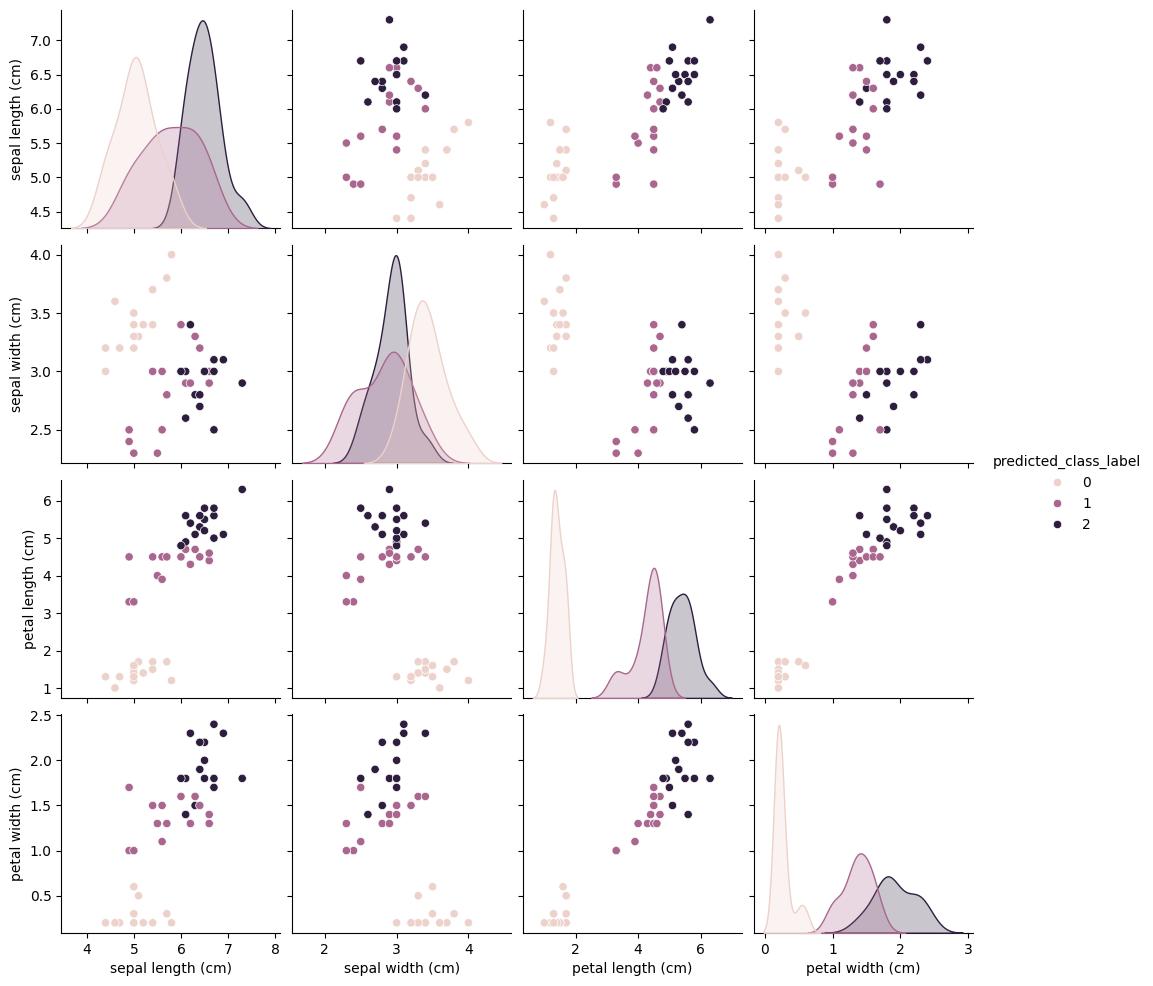
結果の可視化

results1 = X_test.copy()
results1["predicted_class_label"] = predicted_class_label
sns.pairplot(results1, hue="predicted_class_label")

<seaborn.axisgrid.PairGrid at 0x16ff28b90>

../_images/ff4d4d284d77e892a5bb5920aeca731e5727e173319ab084bc9921d8a63ccdd2.png

results1["true_class_label"] = y_test
results1.head(10)

	sepal length (cm)	sepal width (cm)	petal length (cm)	petal width (cm)	predicted_class_label	true_class_label
107	7.3	2.9	6.3	1.8	2	2
63	6.1	2.9	4.7	1.4	1	1
133	6.3	2.8	5.1	1.5	2	2
56	6.3	3.3	4.7	1.6	1	1
127	6.1	3.0	4.9	1.8	2	2
140	6.7	3.1	5.6	2.4	2	2
53	5.5	2.3	4.0	1.3	1	1
69	5.6	2.5	3.9	1.1	1	1
20	5.4	3.4	1.7	0.2	0	0
141	6.9	3.1	5.1	2.3	2	2

classifier.score(X_test,y_test)

0.9555555555555556

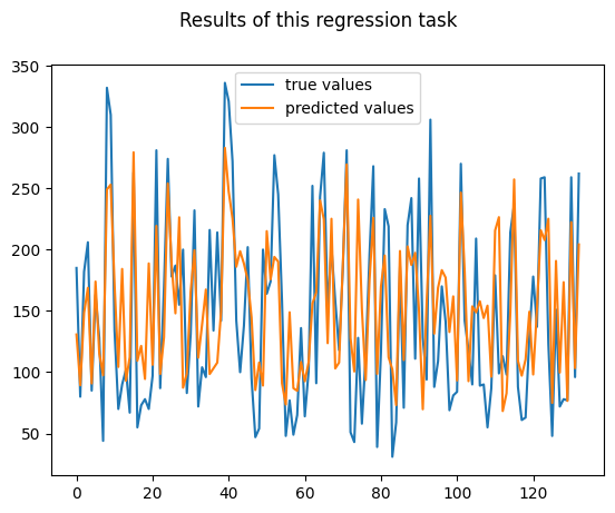
回帰 (Regression)#

与えられた膨大なデータから，それらに対応する数値を予測するタスク．

ここではランダムフォレストを使ったデモを行います．

from sklearn.ensemble import RandomForestRegressor
from sklearn.datasets import load_diabetes

df2 = load_diabetes(as_frame=True)["frame"]
print("---"*10,"raw data","---"*30)
display(df2.head(10))
print("---"*10,"info","---"*30)
print(df2.info())
print("---"*10,"describe","---"*30)
print(df2.describe())

------------------------------ raw data ------------------------------------------------------------------------------------------

	age	sex	bmi	bp	s1	s2	s3	s4	s5	s6	target
0	0.038076	0.050680	0.061696	0.021872	-0.044223	-0.034821	-0.043401	-0.002592	0.019907	-0.017646	151.0
1	-0.001882	-0.044642	-0.051474	-0.026328	-0.008449	-0.019163	0.074412	-0.039493	-0.068332	-0.092204	75.0
2	0.085299	0.050680	0.044451	-0.005670	-0.045599	-0.034194	-0.032356	-0.002592	0.002861	-0.025930	141.0
3	-0.089063	-0.044642	-0.011595	-0.036656	0.012191	0.024991	-0.036038	0.034309	0.022688	-0.009362	206.0
4	0.005383	-0.044642	-0.036385	0.021872	0.003935	0.015596	0.008142	-0.002592	-0.031988	-0.046641	135.0
5	-0.092695	-0.044642	-0.040696	-0.019442	-0.068991	-0.079288	0.041277	-0.076395	-0.041176	-0.096346	97.0
6	-0.045472	0.050680	-0.047163	-0.015999	-0.040096	-0.024800	0.000779	-0.039493	-0.062917	-0.038357	138.0
7	0.063504	0.050680	-0.001895	0.066629	0.090620	0.108914	0.022869	0.017703	-0.035816	0.003064	63.0
8	0.041708	0.050680	0.061696	-0.040099	-0.013953	0.006202	-0.028674	-0.002592	-0.014960	0.011349	110.0
9	-0.070900	-0.044642	0.039062	-0.033213	-0.012577	-0.034508	-0.024993	-0.002592	0.067737	-0.013504	310.0

------------------------------ info ------------------------------------------------------------------------------------------
<class 'pandas.core.frame.DataFrame'>
RangeIndex: 442 entries, 0 to 441
Data columns (total 11 columns):
 #   Column  Non-Null Count  Dtype  
---  ------  --------------  -----  
 0   age     442 non-null    float64
 1   sex     442 non-null    float64
 2   bmi     442 non-null    float64
 3   bp      442 non-null    float64
 4   s1      442 non-null    float64
 5   s2      442 non-null    float64
 6   s3      442 non-null    float64
 7   s4      442 non-null    float64
 8   s5      442 non-null    float64
 9   s6      442 non-null    float64
 10  target  442 non-null    float64
dtypes: float64(11)
memory usage: 38.1 KB
None
------------------------------ describe ------------------------------------------------------------------------------------------
                age           sex           bmi            bp            s1  \
count  4.420000e+02  4.420000e+02  4.420000e+02  4.420000e+02  4.420000e+02   
mean  -2.511817e-19  1.230790e-17 -2.245564e-16 -4.797570e-17 -1.381499e-17   
std    4.761905e-02  4.761905e-02  4.761905e-02  4.761905e-02  4.761905e-02   
min   -1.072256e-01 -4.464164e-02 -9.027530e-02 -1.123988e-01 -1.267807e-01   
25%   -3.729927e-02 -4.464164e-02 -3.422907e-02 -3.665608e-02 -3.424784e-02   
50%    5.383060e-03 -4.464164e-02 -7.283766e-03 -5.670422e-03 -4.320866e-03   
75%    3.807591e-02  5.068012e-02  3.124802e-02  3.564379e-02  2.835801e-02   
max    1.107267e-01  5.068012e-02  1.705552e-01  1.320436e-01  1.539137e-01   

                 s2            s3            s4            s5            s6  \
count  4.420000e+02  4.420000e+02  4.420000e+02  4.420000e+02  4.420000e+02   
mean   3.918434e-17 -5.777179e-18 -9.042540e-18  9.293722e-17  1.130318e-17   
std    4.761905e-02  4.761905e-02  4.761905e-02  4.761905e-02  4.761905e-02   
min   -1.156131e-01 -1.023071e-01 -7.639450e-02 -1.260971e-01 -1.377672e-01   
25%   -3.035840e-02 -3.511716e-02 -3.949338e-02 -3.324559e-02 -3.317903e-02   
50%   -3.819065e-03 -6.584468e-03 -2.592262e-03 -1.947171e-03 -1.077698e-03   
75%    2.984439e-02  2.931150e-02  3.430886e-02  3.243232e-02  2.791705e-02   
max    1.987880e-01  1.811791e-01  1.852344e-01  1.335973e-01  1.356118e-01   

           target  
count  442.000000  
mean   152.133484  
std     77.093005  
min     25.000000  
25%     87.000000  
50%    140.500000  
75%    211.500000  
max    346.000000  

X_train2,X_test2,y_train2,y_test2 = train_test_split(
    df2.iloc[:,:-1], df2["target"],
    test_size=0.3,
    shuffle=True,
    )

regressor = RandomForestRegressor()
regressor.fit(X_train2,y_train2)

RandomForestRegressor()

In a Jupyter environment, please rerun this cell to show the HTML representation or trust the notebook.
On GitHub, the HTML representation is unable to render, please try loading this page with nbviewer.org.

予測結果

predicted_value = regressor.predict(X_test2)
predicted_value

array([130.75,  89.33, 148.52, 168.82,  90.81, 173.92, 115.08,  97.47,
       249.04, 253.01, 171.58, 104.28, 184.22,  93.06, 112.24, 279.37,
       109.33, 121.46,  94.48, 188.71, 106.02, 219.32,  98.57, 128.64,
       253.92, 188.17, 148.01, 226.34,  87.36,  98.86, 165.6 , 199.5 ,
       111.83, 138.82, 167.41,  98.5 , 103.2 , 107.83, 149.75, 283.  ,
       247.3 , 225.36, 186.03, 198.68, 188.52, 175.25, 144.57,  85.44,
       107.83,  89.09, 215.06, 175.73, 194.03, 190.17,  90.92,  73.63,
       148.88,  86.92,  84.84, 108.3 ,  92.55, 108.25, 156.03, 165.02,
       240.1 , 224.75, 123.68, 225.14, 103.08, 107.86, 189.89, 269.44,
       127.77, 100.59, 240.83, 151.35,  93.61, 175.42, 225.9 ,  98.64,
       169.71, 195.16, 112.2 , 102.33,  73.17, 198.85, 109.89, 202.56,
       187.47, 197.38, 150.23,  69.78, 155.9 , 227.56, 131.47, 168.91,
       183.24, 177.13, 132.77, 161.82,  93.27, 246.47, 182.01,  92.69,
       153.69, 148.82, 157.84, 144.17, 154.28,  96.33, 215.61, 226.44,
        68.31,  82.83, 149.05, 257.22, 109.39,  97.14, 110.33, 149.31,
        98.12, 151.62, 215.8 , 207.76, 225.17,  74.94, 190.76,  99.67,
       173.43,  76.58, 222.36, 103.33, 204.19])

結果の可視化

fig = plt.figure()
fig.suptitle("Results of this regression task")
ax = fig.add_subplot(111)
ax.plot(np.arange(len(y_test2)),y_test2,label="true values")
ax.plot(np.arange(len(y_test2)),predicted_value, label="predicted values")
ax.legend()
plt.show()

../_images/080018eab6b69ad9d37bd4e284a70561663ee94746140b31197f6b7d719253d0.png

results2 = X_test2.copy()
results2["predicted_value"] = predicted_value
results2["true_value"] = y_test2
results2.head(10)

	age	sex	bmi	bp	s1	s2	s3	s4	s5	s6	predicted_value	true_value
183	0.045341	0.050680	-0.035307	0.063187	-0.004321	-0.001627	-0.010266	-0.002592	0.015568	0.056912	130.75	185.0
288	0.070769	0.050680	-0.016984	0.021872	0.043837	0.056305	0.037595	-0.002592	-0.070209	-0.017646	89.33	80.0
54	-0.049105	-0.044642	0.025051	0.008101	0.020446	0.017788	0.052322	-0.039493	-0.041176	0.007207	148.52	182.0
365	0.034443	-0.044642	-0.038540	-0.012556	0.009439	0.005262	-0.006584	-0.002592	0.031193	0.098333	168.82	206.0
136	-0.092695	-0.044642	-0.081653	-0.057313	-0.060735	-0.068014	0.048640	-0.076395	-0.066490	-0.021788	90.81	85.0
65	-0.045472	0.050680	-0.024529	0.059744	0.005311	0.014970	-0.054446	0.071210	0.042341	0.015491	173.92	163.0
63	-0.034575	-0.044642	-0.037463	-0.060756	0.020446	0.043466	-0.013948	-0.002592	-0.030748	-0.071494	115.08	128.0
306	0.009016	0.050680	-0.001895	0.021872	-0.038720	-0.024800	-0.006584	-0.039493	-0.039809	-0.013504	97.47	44.0
290	0.059871	0.050680	0.076786	0.025315	0.001183	0.016849	-0.054446	0.034309	0.029935	0.044485	249.04	332.0
254	0.030811	0.050680	0.056307	0.076958	0.049341	-0.012274	-0.036038	0.071210	0.120051	0.090049	253.01	310.0

regressor.score(X_test2,y_test2)

0.47975011322424

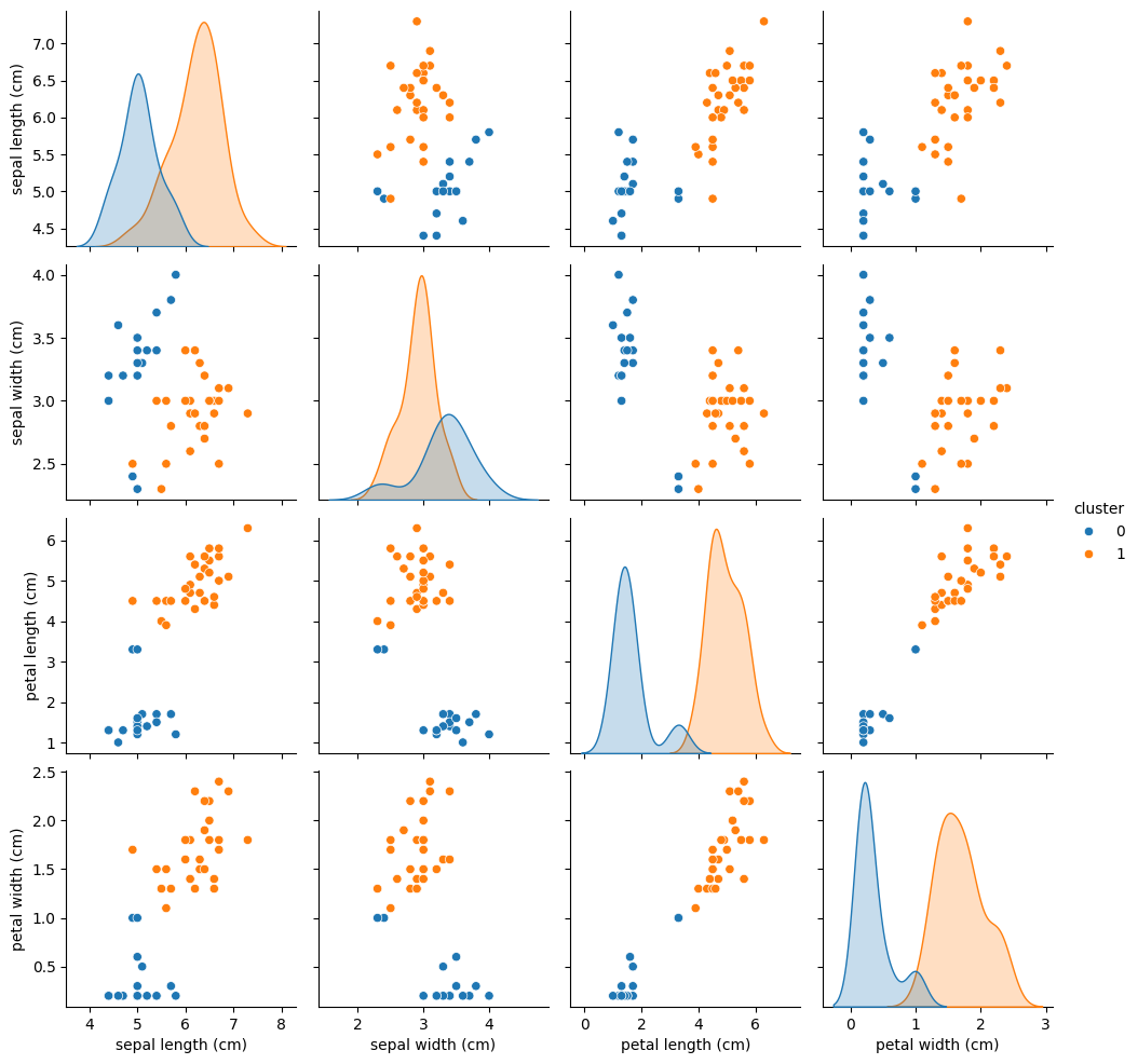
クラスタリング (Clustering)#

与えられた膨大なデータをいくつかのグループに分けるタスク．ここで見つかったグループをクラスターと呼ぶ．

ここではkmeansを使ってデモを行います．

from sklearn.cluster import KMeans

clustering = KMeans(n_clusters=2, n_init="auto")
clustering.fit(X_train)

KMeans(n_clusters=2)

In a Jupyter environment, please rerun this cell to show the HTML representation or trust the notebook.
On GitHub, the HTML representation is unable to render, please try loading this page with nbviewer.org.

clustering.transform(X_train)[:10]

array([[1.92048332, 2.42265007],
       [3.64172282, 0.8523378 ],
       [0.41690734, 4.03925862],
       [5.15481766, 1.25135927],
       [2.92431009, 1.1437106 ],
       [4.55075458, 0.75495562],
       [0.35501261, 4.07961902],
       [0.42548085, 3.9903091 ],
       [0.78770451, 4.32085791],
       [5.2050649 , 1.28253091]])

clustering.predict(X_train)

array([0, 1, 0, 1, 1, 1, 0, 0, 0, 1, 1, 0, 0, 1, 1, 1, 0, 0, 1, 1, 0, 1,
       1, 1, 1, 0, 0, 0, 1, 1, 0, 0, 1, 1, 0, 0, 1, 1, 1, 0, 1, 0, 1, 0,
       1, 1, 0, 1, 1, 1, 1, 0, 1, 1, 1, 1, 0, 1, 0, 1, 1, 1, 1, 1, 1, 1,
       1, 0, 1, 1, 1, 1, 0, 1, 1, 1, 0, 1, 1, 0, 0, 1, 1, 1, 0, 1, 1, 1,
       1, 0, 1, 1, 1, 1, 1, 0, 1, 1, 1, 0, 0, 1, 0, 1, 0], dtype=int32)

clustering.predict(X_test)

array([1, 1, 1, 1, 1, 1, 1, 1, 0, 1, 0, 0, 1, 1, 0, 1, 0, 0, 0, 0, 1, 0,
       1, 1, 1, 1, 1, 0, 1, 0, 1, 1, 1, 0, 1, 0, 0, 0, 0, 1, 1, 0, 1, 1,
       1], dtype=int32)

results1.keys()

Index(['sepal length (cm)', 'sepal width (cm)', 'petal length (cm)',
       'petal width (cm)', 'predicted_class_label', 'true_class_label'],
      dtype='object')

results1["cluster"] = clustering.predict(X_test)
sns.pairplot(
    results1[['sepal length (cm)', 'sepal width (cm)', 'petal length (cm)','petal width (cm)', "cluster"]],
    hue="cluster",
    )

<seaborn.axisgrid.PairGrid at 0x3720589d0>

../_images/b75b8f4ad5536b235f7718b354c65f57a7244400a1e90a4c0bc031218b8112bd.png

results1.head(10)[['sepal length (cm)', 'sepal width (cm)', 'petal length (cm)',
       'petal width (cm)', 'true_class_label',
       'cluster']]

	sepal length (cm)	sepal width (cm)	petal length (cm)	petal width (cm)	true_class_label	cluster
107	7.3	2.9	6.3	1.8	2	1
63	6.1	2.9	4.7	1.4	1	1
133	6.3	2.8	5.1	1.5	2	1
56	6.3	3.3	4.7	1.6	1	1
127	6.1	3.0	4.9	1.8	2	1
140	6.7	3.1	5.6	2.4	2	1
53	5.5	2.3	4.0	1.3	1	1
69	5.6	2.5	3.9	1.1	1	1
20	5.4	3.4	1.7	0.2	0	0
141	6.9	3.1	5.1	2.3	2	1

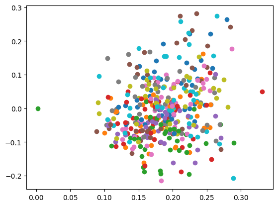
次元削減#

多次元データの情報をできるだけ欠損させずに，より低次元で表現するタスク．

ここではLSI（Latent Semantic Indexing）でデモを行います．

from sklearn.decomposition import TruncatedSVD as LSI
from sklearn.datasets import fetch_20newsgroups
from sklearn.feature_extraction.text import TfidfVectorizer

news = fetch_20newsgroups()
vectorizer = TfidfVectorizer(max_features=2000, stop_words="english")
vectorizer.fit(news.data)

TfidfVectorizer(max_features=2000, stop_words='english')

In a Jupyter environment, please rerun this cell to show the HTML representation or trust the notebook.
On GitHub, the HTML representation is unable to render, please try loading this page with nbviewer.org.

X = vectorizer.transform(news.data)

decomposer = LSI(n_components=2,)
decomposer.fit(X)

TruncatedSVD()

In a Jupyter environment, please rerun this cell to show the HTML representation or trust the notebook.
On GitHub, the HTML representation is unable to render, please try loading this page with nbviewer.org.

embed = decomposer.transform(X)

news_df = pd.DataFrame(embed)
news_df["class"] = news.target
news_df.head()

	0	1	class
0	0.187086	-0.045149	7
1	0.130343	-0.079269	4
2	0.262456	-0.022060	4
3	0.254814	-0.056732	1
4	0.210019	-0.006634	14

for i in range(0,20):
    x = embed[:,0][news.target==i]
    y = embed[:,1][news.target==i]
    plt.scatter(x[:20], y[:20])

../_images/301b6903eb4e94bdcd7dc6921f46f8f5f35ef0214f9bf868b0d1f22848314df6.png

	sepal length (cm)	sepal width (cm)	petal length (cm)	petal width (cm)
0	5.1	3.5	1.4	0.2
1	4.9	3.0	1.4	0.2
2	4.7	3.2	1.3	0.2
3	4.6	3.1	1.5	0.2
4	5.0	3.6	1.4	0.2
5	5.4	3.9	1.7	0.4
6	4.6	3.4	1.4	0.3
7	5.0	3.4	1.5	0.2
8	4.4	2.9	1.4	0.2
9	4.9	3.1	1.5	0.1

	sepal length (cm)	sepal width (cm)	petal length (cm)	petal width (cm)	predicted_class_label	true_class_label
107	7.3	2.9	6.3	1.8	2	2
63	6.1	2.9	4.7	1.4	1	1
133	6.3	2.8	5.1	1.5	2	2
56	6.3	3.3	4.7	1.6	1	1
127	6.1	3.0	4.9	1.8	2	2
140	6.7	3.1	5.6	2.4	2	2
53	5.5	2.3	4.0	1.3	1	1
69	5.6	2.5	3.9	1.1	1	1
20	5.4	3.4	1.7	0.2	0	0
141	6.9	3.1	5.1	2.3	2	2

	sepal length (cm)	sepal width (cm)	petal length (cm)	petal width (cm)	true_class_label	cluster
107	7.3	2.9	6.3	1.8	2	1
63	6.1	2.9	4.7	1.4	1	1
133	6.3	2.8	5.1	1.5	2	1
56	6.3	3.3	4.7	1.6	1	1
127	6.1	3.0	4.9	1.8	2	1
140	6.7	3.1	5.6	2.4	2	1
53	5.5	2.3	4.0	1.3	1	1
69	5.6	2.5	3.9	1.1	1	1
20	5.4	3.4	1.7	0.2	0	0
141	6.9	3.1	5.1	2.3	2	1

	sepal length (cm)	sepal width (cm)	petal length (cm)	petal width (cm)
0	5.1	3.5	1.4	0.2
1	4.9	3.0	1.4	0.2
2	4.7	3.2	1.3	0.2
3	4.6	3.1	1.5	0.2
4	5.0	3.6	1.4	0.2
5	5.4	3.9	1.7	0.4
6	4.6	3.4	1.4	0.3
7	5.0	3.4	1.5	0.2
8	4.4	2.9	1.4	0.2
9	4.9	3.1	1.5	0.1

	sepal length (cm)	sepal width (cm)	petal length (cm)	petal width (cm)	predicted_class_label	true_class_label
107	7.3	2.9	6.3	1.8	2	2
63	6.1	2.9	4.7	1.4	1	1
133	6.3	2.8	5.1	1.5	2	2
56	6.3	3.3	4.7	1.6	1	1
127	6.1	3.0	4.9	1.8	2	2
140	6.7	3.1	5.6	2.4	2	2
53	5.5	2.3	4.0	1.3	1	1
69	5.6	2.5	3.9	1.1	1	1
20	5.4	3.4	1.7	0.2	0	0
141	6.9	3.1	5.1	2.3	2	2

	sepal length (cm)	sepal width (cm)	petal length (cm)	petal width (cm)	true_class_label	cluster
107	7.3	2.9	6.3	1.8	2	1
63	6.1	2.9	4.7	1.4	1	1
133	6.3	2.8	5.1	1.5	2	1
56	6.3	3.3	4.7	1.6	1	1
127	6.1	3.0	4.9	1.8	2	1
140	6.7	3.1	5.6	2.4	2	1
53	5.5	2.3	4.0	1.3	1	1
69	5.6	2.5	3.9	1.1	1	1
20	5.4	3.4	1.7	0.2	0	0
141	6.9	3.1	5.1	2.3	2	1

Scikit-Learn overview

Contents

Scikit-Learn overview#

クラス分類 (Classification)#

回帰 (Regression)#

クラスタリング (Clustering)#

次元削減#

	sepal length (cm)	sepal width (cm)	petal length (cm)	petal width (cm)
0	5.1	3.5	1.4	0.2
1	4.9	3.0	1.4	0.2
2	4.7	3.2	1.3	0.2
3	4.6	3.1	1.5	0.2
4	5.0	3.6	1.4	0.2
5	5.4	3.9	1.7	0.4
6	4.6	3.4	1.4	0.3
7	5.0	3.4	1.5	0.2
8	4.4	2.9	1.4	0.2
9	4.9	3.1	1.5	0.1

	sepal length (cm)	sepal width (cm)	petal length (cm)	petal width (cm)	predicted_class_label	true_class_label
107	7.3	2.9	6.3	1.8	2	2
63	6.1	2.9	4.7	1.4	1	1
133	6.3	2.8	5.1	1.5	2	2
56	6.3	3.3	4.7	1.6	1	1
127	6.1	3.0	4.9	1.8	2	2
140	6.7	3.1	5.6	2.4	2	2
53	5.5	2.3	4.0	1.3	1	1
69	5.6	2.5	3.9	1.1	1	1
20	5.4	3.4	1.7	0.2	0	0
141	6.9	3.1	5.1	2.3	2	2

	sepal length (cm)	sepal width (cm)	petal length (cm)	petal width (cm)	true_class_label	cluster
107	7.3	2.9	6.3	1.8	2	1
63	6.1	2.9	4.7	1.4	1	1
133	6.3	2.8	5.1	1.5	2	1
56	6.3	3.3	4.7	1.6	1	1
127	6.1	3.0	4.9	1.8	2	1
140	6.7	3.1	5.6	2.4	2	1
53	5.5	2.3	4.0	1.3	1	1
69	5.6	2.5	3.9	1.1	1	1
20	5.4	3.4	1.7	0.2	0	0
141	6.9	3.1	5.1	2.3	2	1