パルマーペンギンデータセットを例にPyTorchの使い方を学ぼう#
ニューラルネットワークの実装のためのライブラリ「PyTorch」の使い方を,penguinデータセットのクラス分類を例に学ぼう.
import torch
import torch.nn as nn
import torch.nn.functional as F
from sklearn.preprocessing import StandardScaler
import pandas as pd
import numpy as np
import random
import os
SEED = 20220725

# seed function for reproducibility
def set_seed(seed: int=0):
    random.seed(seed)
    np.random.seed(seed)
    os.environ["PYTHONHASHSEED"] = str(seed)
    torch.manual_seed(seed)
    torch.cuda.manual_seed(seed)
    torch.backends.cudnn.deterministic = True
    torch.backends.cudnn.benchmark = False

set_seed(SEED)
SECTION 1 : 学習用データのロードとセットアップ#

オリジンデータをもとに2つのファイルに分けたデータセット 。
penguin-clean-train.csv = 学習用データセット、オリジナルデータから70%使用。
penguin-clean-test.csv = テスト用データセット、オリジナルデータから30%抽出
SECTION 1 : Load and setup data for training
the datasets separated in two files from originai datasets:
penguin-clean-train.csv = datasets for training purpose, 70% from the original data
penguin-clean-test.csv = datasets for testing purpose, 30% from the original data
Section 1.1 Data Loading#
データセットは前処理済みのものが既にあるので、これを直接利用する rianrajagede/penguin-python
en2ja = {
    "species": "ペンギンの種類",
    "island": "生息する島",
    "bill_length_mm": "クチバシの長さ",
    "bill_depth_mm":"クチバシの厚み",
    "flipper_length_mm": "翼の長さ",
    "body_mass_g": "体重",
    "sex": "性別",
    "year": "調査年",
}
#load

dataset_url = "https://raw.githubusercontent.com/rianrajagede/penguin-python/master/Datasets/penguins-clean-all.csv"
training_url = "https://raw.githubusercontent.com/rianrajagede/penguin-python/master/Datasets/penguins-clean-train.csv"
test_url = "https://raw.githubusercontent.com/rianrajagede/penguin-python/master/Datasets/penguins-clean-test.csv"
# datatrain = pd.read_csv('../Datasets/penguins-clean-train.csv')
df_train = pd.read_csv(training_url)
df_train.shape
(240, 5)
df_train_ja = df_train.copy()
df_train_ja.columns = [en2ja[key] for key in df_train_ja.columns]
df_train_ja
| ペンギンの種類 | クチバシの長さ | クチバシの厚み | 翼の長さ | 体重 | |
|---|---|---|---|---|---|
| 0 | Gentoo | 46.2 | 14.5 | 209 | 4800 |
| 1 | Gentoo | 43.6 | 13.9 | 217 | 4900 |
| 2 | Gentoo | 45.3 | 13.7 | 210 | 4300 |
| 3 | Gentoo | 53.4 | 15.8 | 219 | 5500 |
| 4 | Adelie | 40.6 | 18.8 | 193 | 3800 |
| ... | ... | ... | ... | ... | ... |
| 235 | Gentoo | 46.8 | 15.4 | 215 | 5150 |
| 236 | Gentoo | 46.6 | 14.2 | 210 | 4850 |
| 237 | Gentoo | 43.5 | 14.2 | 220 | 4700 |
| 238 | Gentoo | 46.9 | 14.6 | 222 | 4875 |
| 239 | Chinstrap | 50.7 | 19.7 | 203 | 4050 |
240 rows × 5 columns
#Section 1.2 Preprocessing

#change string value to numeric
df_train.loc[df_train['species']=='Adelie', 'species']=0
df_train.loc[df_train['species']=='Gentoo', 'species']=1
df_train.loc[df_train['species']=='Chinstrap', 'species']=2
df_train = df_train.apply(pd.to_numeric)

#change dataframe to array
df_array = df_train.values

#split x and y (feature and target)
X_train = df_array[:,1:]
y_train = df_array[:,0]

#standardize
#palmer-penguin dataset has varying scales
scaler = StandardScaler()
X_train = scaler.fit_transform(X_train)
SECTION 2 : モデルの構築と学習#
隠れ層を1層持つ、多層パーセプトロンモデル。
入力層:4ニューロン、Palmer Penguinデータセットからの特徴を表す。
隠れ層:20ニューロン、ReLUで活性化
出力層:3ニューロン、種の数を表す、Softmax Layer
最適化器 = 確率的勾配降下法、バッチサイズなし
損失関数 = カテゴリクロスエントロピー
学習率 = 0.01
エポック = 50
SECTION 2 : Build and Train Model
Multilayer perceptron model, with one hidden layer.
input layer : 4 neuron, represents the feature from Palmer Penguin dataset
hidden layer : 20 neuron, activation using ReLU output layer : 3 neuron, represents the number of species, Softmax Layer optimizer = stochastic gradient descent with no batch-size
loss function = categorical cross entropy
learning rate = 0.01 #hyperparameters hl = 20 lr = 0.01 num_epoch = 100
epoch = 50
#hyperparameters
hl = 20
lr = 0.01
num_epoch = 100
ネットワークはnn.Sequentialを使って作るパターンと,nn.Moduleを継承したクラスを作るパターンがある.
mynet = nn.Sequential(
    nn.Linear(4, 20,),
    nn.ReLU(),
    nn.Linear(20, 3),
    nn.Softmax(dim=1)
)
#build model
class Net(nn.Module):
    def __init__(self):
        super().__init__()
        self.fc1 = nn.Linear(4, hl)
        self.fc2 = nn.Linear(hl, 3)

    def forward(self, x):
        x = F.relu(self.fc1(x))
        x = self.fc2(x)
        return x

net = Net()
#choose optimizer and loss function
criterion = nn.CrossEntropyLoss()
optimizer = torch.optim.SGD(net.parameters(), lr=lr)

X_train = torch.from_numpy(X_train).float()
y_train = torch.from_numpy(y_train).long()
print("training data:",type(X_train), X_train.shape, X_train.dtype)
print("test data:", type(y_train), y_train.shape, y_train.dtype)
training data: <class 'torch.Tensor'> torch.Size([240, 4]) torch.float32
test data: <class 'torch.Tensor'> torch.Size([240]) torch.int64
net.eval()
print(net.training
)
net.train()
print(net.training
)
False
True
訓練ループ
# logging
logs = {"loss":[], "acc":[]}

#train
if torch.cuda.is_available():
  net = net.to("cuda:0")
  X_train = X_train.to("cuda:0")
  y_train = y_train.to("cuda:0")

for epoch in range(num_epoch):

    #feedforward - backprop
    # 勾配の初期化
    optimizer.zero_grad()
    # フォワードプロップ。順伝搬
    out = net(X_train)
    # 損失関数の計算
    loss = criterion(out, y_train)
    # 逆伝搬して、各パラメータの勾配を求める
    loss.backward()
    # 勾配を使って学習可能パラメータの値を更新
    optimizer.step()

    with torch.no_grad():
        acc = 100 * torch.sum(y_train==torch.max(out.data, 1)[1]).double() / len(y_train)
    print ('Epoch [%d/%d] Loss: %.4f   Acc: %.4f'
                   %(epoch+1, num_epoch, loss.item(), acc.item()))

    # logging
    logs["loss"] += [loss.cpu().detach().item()]
    logs["acc"]  += [acc.cpu().detach().item()]
Epoch [1/100] Loss: 1.1014   Acc: 42.9167
Epoch [2/100] Loss: 1.0938   Acc: 44.1667
Epoch [3/100] Loss: 1.0864   Acc: 46.2500
Epoch [4/100] Loss: 1.0790   Acc: 49.1667
Epoch [5/100] Loss: 1.0718   Acc: 51.6667
Epoch [6/100] Loss: 1.0646   Acc: 52.5000
Epoch [7/100] Loss: 1.0575   Acc: 55.4167
Epoch [8/100] Loss: 1.0505   Acc: 55.4167
Epoch [9/100] Loss: 1.0436   Acc: 59.1667
Epoch [10/100] Loss: 1.0367   Acc: 60.4167
Epoch [11/100] Loss: 1.0300   Acc: 62.5000
Epoch [12/100] Loss: 1.0233   Acc: 66.2500
Epoch [13/100] Loss: 1.0167   Acc: 67.5000
Epoch [14/100] Loss: 1.0102   Acc: 68.3333
Epoch [15/100] Loss: 1.0037   Acc: 70.4167
Epoch [16/100] Loss: 0.9973   Acc: 71.2500
Epoch [17/100] Loss: 0.9910   Acc: 72.9167
Epoch [18/100] Loss: 0.9848   Acc: 73.7500
Epoch [19/100] Loss: 0.9786   Acc: 74.1667
Epoch [20/100] Loss: 0.9725   Acc: 75.8333
Epoch [21/100] Loss: 0.9664   Acc: 75.8333
Epoch [22/100] Loss: 0.9604   Acc: 76.2500
Epoch [23/100] Loss: 0.9545   Acc: 76.2500
Epoch [24/100] Loss: 0.9486   Acc: 76.2500
Epoch [25/100] Loss: 0.9428   Acc: 77.0833
Epoch [26/100] Loss: 0.9371   Acc: 77.5000
Epoch [27/100] Loss: 0.9314   Acc: 77.9167
Epoch [28/100] Loss: 0.9257   Acc: 77.9167
Epoch [29/100] Loss: 0.9202   Acc: 78.3333
Epoch [30/100] Loss: 0.9146   Acc: 78.3333
Epoch [31/100] Loss: 0.9092   Acc: 78.3333
Epoch [32/100] Loss: 0.9038   Acc: 78.3333
Epoch [33/100] Loss: 0.8984   Acc: 78.3333
Epoch [34/100] Loss: 0.8931   Acc: 78.3333
Epoch [35/100] Loss: 0.8878   Acc: 78.3333
Epoch [36/100] Loss: 0.8826   Acc: 78.3333
Epoch [37/100] Loss: 0.8775   Acc: 78.3333
Epoch [38/100] Loss: 0.8723   Acc: 78.3333
Epoch [39/100] Loss: 0.8673   Acc: 78.7500
Epoch [40/100] Loss: 0.8623   Acc: 78.7500
Epoch [41/100] Loss: 0.8573   Acc: 78.7500
Epoch [42/100] Loss: 0.8524   Acc: 78.7500
Epoch [43/100] Loss: 0.8475   Acc: 78.7500
Epoch [44/100] Loss: 0.8427   Acc: 78.7500
Epoch [45/100] Loss: 0.8379   Acc: 78.7500
Epoch [46/100] Loss: 0.8331   Acc: 79.1667
Epoch [47/100] Loss: 0.8284   Acc: 79.1667
Epoch [48/100] Loss: 0.8238   Acc: 79.1667
Epoch [49/100] Loss: 0.8192   Acc: 79.1667
Epoch [50/100] Loss: 0.8146   Acc: 79.1667
Epoch [51/100] Loss: 0.8101   Acc: 79.5833
Epoch [52/100] Loss: 0.8056   Acc: 79.5833
Epoch [53/100] Loss: 0.8012   Acc: 80.0000
Epoch [54/100] Loss: 0.7968   Acc: 80.0000
Epoch [55/100] Loss: 0.7924   Acc: 80.0000
Epoch [56/100] Loss: 0.7881   Acc: 80.0000
Epoch [57/100] Loss: 0.7838   Acc: 80.0000
Epoch [58/100] Loss: 0.7795   Acc: 80.0000
Epoch [59/100] Loss: 0.7753   Acc: 80.0000
Epoch [60/100] Loss: 0.7712   Acc: 80.0000
Epoch [61/100] Loss: 0.7670   Acc: 80.0000
Epoch [62/100] Loss: 0.7629   Acc: 80.0000
Epoch [63/100] Loss: 0.7589   Acc: 80.0000
Epoch [64/100] Loss: 0.7548   Acc: 80.0000
Epoch [65/100] Loss: 0.7508   Acc: 80.0000
Epoch [66/100] Loss: 0.7469   Acc: 80.0000
Epoch [67/100] Loss: 0.7430   Acc: 80.0000
Epoch [68/100] Loss: 0.7391   Acc: 80.0000
Epoch [69/100] Loss: 0.7352   Acc: 80.0000
Epoch [70/100] Loss: 0.7314   Acc: 80.0000
Epoch [71/100] Loss: 0.7276   Acc: 80.0000
Epoch [72/100] Loss: 0.7239   Acc: 80.0000
Epoch [73/100] Loss: 0.7202   Acc: 80.0000
Epoch [74/100] Loss: 0.7165   Acc: 80.0000
Epoch [75/100] Loss: 0.7128   Acc: 80.0000
Epoch [76/100] Loss: 0.7092   Acc: 80.0000
Epoch [77/100] Loss: 0.7056   Acc: 80.0000
Epoch [78/100] Loss: 0.7021   Acc: 80.0000
Epoch [79/100] Loss: 0.6985   Acc: 80.0000
Epoch [80/100] Loss: 0.6950   Acc: 80.0000
Epoch [81/100] Loss: 0.6916   Acc: 80.0000
Epoch [82/100] Loss: 0.6882   Acc: 80.0000
Epoch [83/100] Loss: 0.6847   Acc: 80.0000
Epoch [84/100] Loss: 0.6814   Acc: 80.0000
Epoch [85/100] Loss: 0.6780   Acc: 80.0000
Epoch [86/100] Loss: 0.6747   Acc: 80.0000
Epoch [87/100] Loss: 0.6714   Acc: 80.0000
Epoch [88/100] Loss: 0.6682   Acc: 80.0000
Epoch [89/100] Loss: 0.6650   Acc: 80.0000
Epoch [90/100] Loss: 0.6618   Acc: 80.0000
Epoch [91/100] Loss: 0.6586   Acc: 80.0000
Epoch [92/100] Loss: 0.6555   Acc: 80.0000
Epoch [93/100] Loss: 0.6523   Acc: 80.0000
Epoch [94/100] Loss: 0.6493   Acc: 80.0000
Epoch [95/100] Loss: 0.6462   Acc: 80.0000
Epoch [96/100] Loss: 0.6432   Acc: 80.0000
Epoch [97/100] Loss: 0.6402   Acc: 80.0000
Epoch [98/100] Loss: 0.6372   Acc: 80.0000
Epoch [99/100] Loss: 0.6342   Acc: 80.0000
Epoch [100/100] Loss: 0.6313   Acc: 80.0000
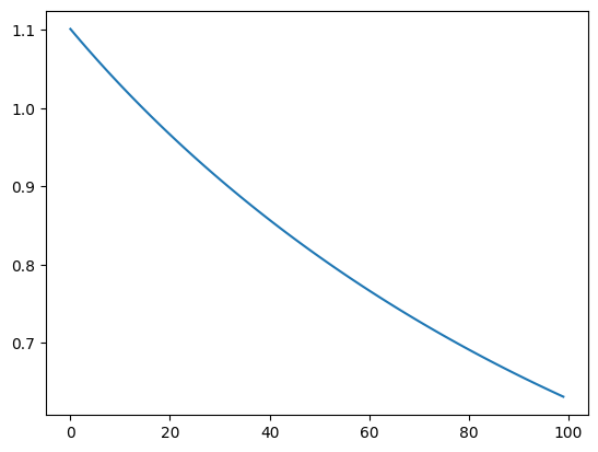
学習中の損失関数のモニタリング
pd.DataFrame(logs)["loss"].plot()
<Axes: >
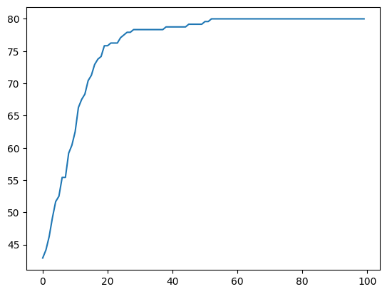
学習中の正答率のモニタリング
pd.DataFrame(logs)["acc"].plot()
<Axes: >
SECTION 3 : モデルの評価#
#load
df_test = pd.read_csv(test_url)

#change string value to numeric
df_test.loc[df_test['species']=='Adelie', 'species']=0
df_test.loc[df_test['species']=='Gentoo', 'species']=1
df_test.loc[df_test['species']=='Chinstrap', 'species']=2
df_test = df_test.apply(pd.to_numeric)

#change dataframe to array
df_test_array = df_test.values

#split x and y (feature and target)
X_test = df_test_array[:,1:]
y_test = df_test_array[:,0]

#standardization
X_test = scaler.transform(X_test)

#get prediction
X_test = torch.Tensor(X_test).float()
y_test = torch.Tensor(y_test).long()

# 必要ならばCPUからGPUへ配列を移動
#X_test = X_test.to(X_train.device)
#y_test = y_test.to(y_train.device)

if torch.cuda.is_available():
  X_test = X_test.cuda()
  y_test = y_test.cuda()

#テストデータに対するクラスラベルの予測
out = net.forward(X_test)#.softmax(1)
_, predicted = torch.max(out.data, 1)

#get accuration
print('Accuracy of the network %.4f %%' % (100 * torch.sum(y_test==predicted).double() / len(y_test)))
Accuracy of the network 80.3922 %
[課題1] 入力層の次元数と隠れ層の次元数とクラス数を__init__の引数で変更できるようにNetクラスを修正せよ。#
Show code cell source
class FixedNet(nn.Module):

    def __init__(self, num_features, hidden_size, num_class):
        super().__init__()
        self.fc1 = nn.Linear(num_features, hidden_size)
        self.fc2 = nn.Linear(hidden_size, num_class)

    def forward(self, x):
        x = F.relu(self.fc1(x))
        x = self.fc2(x)
        return x

num_features = X_train.shape[1]
hidden_size = 100
num_class = 3
fixed_net = FixedNet(num_features,hidden_size, num_class)
fixed_net
FixedNet(
  (fc1): Linear(in_features=4, out_features=100, bias=True)
  (fc2): Linear(in_features=100, out_features=3, bias=True)
)
[課題2] 課題1で作ったクラスを使って,クラス数をそのままに隠れ層の次元数を100にして200エポック訓練せよ.また,その際のtestデータの正答率を示せ.この際、set_seedを使いSEEDを1111に固定する事.#
Show code cell source
set_seed(1111)
net = FixedNet(num_features,hidden_size, num_class)
#choose optimizer and loss function
criterion = nn.CrossEntropyLoss()
optimizer = torch.optim.SGD(net.parameters(), lr=lr)

# 訓練のコード

# 評価のコード
[課題3] ペンギンデータのクラス分類を行うニューラルネットワークを作れ。ただし、ニューラルネットワークの隠れ層は5層で、それぞれが100次元のネットワークを作成せよ。また、このニューラルネットワークの活性化関数はすべてtanhである。この隠れ層をまとめたsequentialをfeature_extractorという変数にせよ。出力層は3クラス分類を行うために次元数は3にする。#
class TanhNet(nn.Module):
  def __init__(self, hidden_size=100, n_class=3):
    super().__init__()
    self.feature_extractor = nn.Sequential(
          nn.Linear(4, hidden_size), # 1
          nn.Tanh(),
          nn.Linear(hidden_size, hidden_size), # 2
          nn.Tanh(),
          ... # 3
          ... # 4
          ... # 5
      )
    self.classifier = nn.Linear(hidden_size, n_class)

  def forward(self,x):
    x = self.feature_extractor(x)
    return self.classifier(x)
  Cell In[19], line 9
    ... # 3
    ^
SyntaxError: invalid syntax. Perhaps you forgot a comma?
a = TanhNet()
#a(X_train.cpu())
a
TanhNet(
  (feature_extractor): Sequential(
    (0): Linear(in_features=4, out_features=100, bias=True)
    (1): Tanh()
    (2): Linear(in_features=100, out_features=100, bias=True)
    (3): Tanh()
  )
  (classifier): Linear(in_features=100, out_features=3, bias=True)
)