Pandas#
pandasはデータ解析・機械学習のためのデータ形式を提供するライブラリです。
特に使うのはDataFrameです。
DataFrameは行列を扱うクラスで、DataFrameを使えばExcelのSpreadsheetのように見やすいデータ解析ができます。
import numpy as np
from sklearn import datasets
import pandas as pd
scikit-learnとは
scikit-learn (sklearn)とは、Pythonの機械学習ライブラリのde facto standardだと言える有名なライブラリです。
このライブラリには、有名な機械学習手法を実装したクラスだけでなく、データをダウンロードして読み込む関数や、データの前処理を行う関数などが含まれています。
データの読み込み#
sklearnからデータを読み込む#
sklearn.datasetsはデータ読み込みパッケージです。
このパッケージの中にはload_*という関数がいくつか用意されていて、これらの関数を使うとデータセットを読み込むことができます。
また、この関数で得られるデータセットは辞書型になっています。
data: データ本体が入っています。型はnp.arrayです。
target: データのlabel(クラス)が入っています。
target_names: labelの本当の名前が入っています。
feature_names: 特徴の名前が入っています。
iris = datasets.load_iris()
iris
Show code cell output
{'data': array([[5.1, 3.5, 1.4, 0.2],
        [4.9, 3. , 1.4, 0.2],
        [4.7, 3.2, 1.3, 0.2],
        [4.6, 3.1, 1.5, 0.2],
        [5. , 3.6, 1.4, 0.2],
        [5.4, 3.9, 1.7, 0.4],
        [4.6, 3.4, 1.4, 0.3],
        [5. , 3.4, 1.5, 0.2],
        [4.4, 2.9, 1.4, 0.2],
        [4.9, 3.1, 1.5, 0.1],
        [5.4, 3.7, 1.5, 0.2],
        [4.8, 3.4, 1.6, 0.2],
        [4.8, 3. , 1.4, 0.1],
        [4.3, 3. , 1.1, 0.1],
        [5.8, 4. , 1.2, 0.2],
        [5.7, 4.4, 1.5, 0.4],
        [5.4, 3.9, 1.3, 0.4],
        [5.1, 3.5, 1.4, 0.3],
        [5.7, 3.8, 1.7, 0.3],
        [5.1, 3.8, 1.5, 0.3],
        [5.4, 3.4, 1.7, 0.2],
        [5.1, 3.7, 1.5, 0.4],
        [4.6, 3.6, 1. , 0.2],
        [5.1, 3.3, 1.7, 0.5],
        [4.8, 3.4, 1.9, 0.2],
        [5. , 3. , 1.6, 0.2],
        [5. , 3.4, 1.6, 0.4],
        [5.2, 3.5, 1.5, 0.2],
        [5.2, 3.4, 1.4, 0.2],
        [4.7, 3.2, 1.6, 0.2],
        [4.8, 3.1, 1.6, 0.2],
        [5.4, 3.4, 1.5, 0.4],
        [5.2, 4.1, 1.5, 0.1],
        [5.5, 4.2, 1.4, 0.2],
        [4.9, 3.1, 1.5, 0.2],
        [5. , 3.2, 1.2, 0.2],
        [5.5, 3.5, 1.3, 0.2],
        [4.9, 3.6, 1.4, 0.1],
        [4.4, 3. , 1.3, 0.2],
        [5.1, 3.4, 1.5, 0.2],
        [5. , 3.5, 1.3, 0.3],
        [4.5, 2.3, 1.3, 0.3],
        [4.4, 3.2, 1.3, 0.2],
        [5. , 3.5, 1.6, 0.6],
        [5.1, 3.8, 1.9, 0.4],
        [4.8, 3. , 1.4, 0.3],
        [5.1, 3.8, 1.6, 0.2],
        [4.6, 3.2, 1.4, 0.2],
        [5.3, 3.7, 1.5, 0.2],
        [5. , 3.3, 1.4, 0.2],
        [7. , 3.2, 4.7, 1.4],
        [6.4, 3.2, 4.5, 1.5],
        [6.9, 3.1, 4.9, 1.5],
        [5.5, 2.3, 4. , 1.3],
        [6.5, 2.8, 4.6, 1.5],
        [5.7, 2.8, 4.5, 1.3],
        [6.3, 3.3, 4.7, 1.6],
        [4.9, 2.4, 3.3, 1. ],
        [6.6, 2.9, 4.6, 1.3],
        [5.2, 2.7, 3.9, 1.4],
        [5. , 2. , 3.5, 1. ],
        [5.9, 3. , 4.2, 1.5],
        [6. , 2.2, 4. , 1. ],
        [6.1, 2.9, 4.7, 1.4],
        [5.6, 2.9, 3.6, 1.3],
        [6.7, 3.1, 4.4, 1.4],
        [5.6, 3. , 4.5, 1.5],
        [5.8, 2.7, 4.1, 1. ],
        [6.2, 2.2, 4.5, 1.5],
        [5.6, 2.5, 3.9, 1.1],
        [5.9, 3.2, 4.8, 1.8],
        [6.1, 2.8, 4. , 1.3],
        [6.3, 2.5, 4.9, 1.5],
        [6.1, 2.8, 4.7, 1.2],
        [6.4, 2.9, 4.3, 1.3],
        [6.6, 3. , 4.4, 1.4],
        [6.8, 2.8, 4.8, 1.4],
        [6.7, 3. , 5. , 1.7],
        [6. , 2.9, 4.5, 1.5],
        [5.7, 2.6, 3.5, 1. ],
        [5.5, 2.4, 3.8, 1.1],
        [5.5, 2.4, 3.7, 1. ],
        [5.8, 2.7, 3.9, 1.2],
        [6. , 2.7, 5.1, 1.6],
        [5.4, 3. , 4.5, 1.5],
        [6. , 3.4, 4.5, 1.6],
        [6.7, 3.1, 4.7, 1.5],
        [6.3, 2.3, 4.4, 1.3],
        [5.6, 3. , 4.1, 1.3],
        [5.5, 2.5, 4. , 1.3],
        [5.5, 2.6, 4.4, 1.2],
        [6.1, 3. , 4.6, 1.4],
        [5.8, 2.6, 4. , 1.2],
        [5. , 2.3, 3.3, 1. ],
        [5.6, 2.7, 4.2, 1.3],
        [5.7, 3. , 4.2, 1.2],
        [5.7, 2.9, 4.2, 1.3],
        [6.2, 2.9, 4.3, 1.3],
        [5.1, 2.5, 3. , 1.1],
        [5.7, 2.8, 4.1, 1.3],
        [6.3, 3.3, 6. , 2.5],
        [5.8, 2.7, 5.1, 1.9],
        [7.1, 3. , 5.9, 2.1],
        [6.3, 2.9, 5.6, 1.8],
        [6.5, 3. , 5.8, 2.2],
        [7.6, 3. , 6.6, 2.1],
        [4.9, 2.5, 4.5, 1.7],
        [7.3, 2.9, 6.3, 1.8],
        [6.7, 2.5, 5.8, 1.8],
        [7.2, 3.6, 6.1, 2.5],
        [6.5, 3.2, 5.1, 2. ],
        [6.4, 2.7, 5.3, 1.9],
        [6.8, 3. , 5.5, 2.1],
        [5.7, 2.5, 5. , 2. ],
        [5.8, 2.8, 5.1, 2.4],
        [6.4, 3.2, 5.3, 2.3],
        [6.5, 3. , 5.5, 1.8],
        [7.7, 3.8, 6.7, 2.2],
        [7.7, 2.6, 6.9, 2.3],
        [6. , 2.2, 5. , 1.5],
        [6.9, 3.2, 5.7, 2.3],
        [5.6, 2.8, 4.9, 2. ],
        [7.7, 2.8, 6.7, 2. ],
        [6.3, 2.7, 4.9, 1.8],
        [6.7, 3.3, 5.7, 2.1],
        [7.2, 3.2, 6. , 1.8],
        [6.2, 2.8, 4.8, 1.8],
        [6.1, 3. , 4.9, 1.8],
        [6.4, 2.8, 5.6, 2.1],
        [7.2, 3. , 5.8, 1.6],
        [7.4, 2.8, 6.1, 1.9],
        [7.9, 3.8, 6.4, 2. ],
        [6.4, 2.8, 5.6, 2.2],
        [6.3, 2.8, 5.1, 1.5],
        [6.1, 2.6, 5.6, 1.4],
        [7.7, 3. , 6.1, 2.3],
        [6.3, 3.4, 5.6, 2.4],
        [6.4, 3.1, 5.5, 1.8],
        [6. , 3. , 4.8, 1.8],
        [6.9, 3.1, 5.4, 2.1],
        [6.7, 3.1, 5.6, 2.4],
        [6.9, 3.1, 5.1, 2.3],
        [5.8, 2.7, 5.1, 1.9],
        [6.8, 3.2, 5.9, 2.3],
        [6.7, 3.3, 5.7, 2.5],
        [6.7, 3. , 5.2, 2.3],
        [6.3, 2.5, 5. , 1.9],
        [6.5, 3. , 5.2, 2. ],
        [6.2, 3.4, 5.4, 2.3],
        [5.9, 3. , 5.1, 1.8]]),
 'target': array([0, 0, 0, 0, 0, 0, 0, 0, 0, 0, 0, 0, 0, 0, 0, 0, 0, 0, 0, 0, 0, 0,
        0, 0, 0, 0, 0, 0, 0, 0, 0, 0, 0, 0, 0, 0, 0, 0, 0, 0, 0, 0, 0, 0,
        0, 0, 0, 0, 0, 0, 1, 1, 1, 1, 1, 1, 1, 1, 1, 1, 1, 1, 1, 1, 1, 1,
        1, 1, 1, 1, 1, 1, 1, 1, 1, 1, 1, 1, 1, 1, 1, 1, 1, 1, 1, 1, 1, 1,
        1, 1, 1, 1, 1, 1, 1, 1, 1, 1, 1, 1, 2, 2, 2, 2, 2, 2, 2, 2, 2, 2,
        2, 2, 2, 2, 2, 2, 2, 2, 2, 2, 2, 2, 2, 2, 2, 2, 2, 2, 2, 2, 2, 2,
        2, 2, 2, 2, 2, 2, 2, 2, 2, 2, 2, 2, 2, 2, 2, 2, 2, 2]),
 'frame': None,
 'target_names': array(['setosa', 'versicolor', 'virginica'], dtype='<U10'),
 'DESCR': '.. _iris_dataset:\n\nIris plants dataset\n--------------------\n\n**Data Set Characteristics:**\n\n:Number of Instances: 150 (50 in each of three classes)\n:Number of Attributes: 4 numeric, predictive attributes and the class\n:Attribute Information:\n    - sepal length in cm\n    - sepal width in cm\n    - petal length in cm\n    - petal width in cm\n    - class:\n            - Iris-Setosa\n            - Iris-Versicolour\n            - Iris-Virginica\n\n:Summary Statistics:\n\n============== ==== ==== ======= ===== ====================\n                Min  Max   Mean    SD   Class Correlation\n============== ==== ==== ======= ===== ====================\nsepal length:   4.3  7.9   5.84   0.83    0.7826\nsepal width:    2.0  4.4   3.05   0.43   -0.4194\npetal length:   1.0  6.9   3.76   1.76    0.9490  (high!)\npetal width:    0.1  2.5   1.20   0.76    0.9565  (high!)\n============== ==== ==== ======= ===== ====================\n\n:Missing Attribute Values: None\n:Class Distribution: 33.3% for each of 3 classes.\n:Creator: R.A. Fisher\n:Donor: Michael Marshall (MARSHALL%PLU@io.arc.nasa.gov)\n:Date: July, 1988\n\nThe famous Iris database, first used by Sir R.A. Fisher. The dataset is taken\nfrom Fisher\'s paper. Note that it\'s the same as in R, but not as in the UCI\nMachine Learning Repository, which has two wrong data points.\n\nThis is perhaps the best known database to be found in the\npattern recognition literature.  Fisher\'s paper is a classic in the field and\nis referenced frequently to this day.  (See Duda & Hart, for example.)  The\ndata set contains 3 classes of 50 instances each, where each class refers to a\ntype of iris plant.  One class is linearly separable from the other 2; the\nlatter are NOT linearly separable from each other.\n\n|details-start|\n**References**\n|details-split|\n\n- Fisher, R.A. "The use of multiple measurements in taxonomic problems"\n  Annual Eugenics, 7, Part II, 179-188 (1936); also in "Contributions to\n  Mathematical Statistics" (John Wiley, NY, 1950).\n- Duda, R.O., & Hart, P.E. (1973) Pattern Classification and Scene Analysis.\n  (Q327.D83) John Wiley & Sons.  ISBN 0-471-22361-1.  See page 218.\n- Dasarathy, B.V. (1980) "Nosing Around the Neighborhood: A New System\n  Structure and Classification Rule for Recognition in Partially Exposed\n  Environments".  IEEE Transactions on Pattern Analysis and Machine\n  Intelligence, Vol. PAMI-2, No. 1, 67-71.\n- Gates, G.W. (1972) "The Reduced Nearest Neighbor Rule".  IEEE Transactions\n  on Information Theory, May 1972, 431-433.\n- See also: 1988 MLC Proceedings, 54-64.  Cheeseman et al"s AUTOCLASS II\n  conceptual clustering system finds 3 classes in the data.\n- Many, many more ...\n\n|details-end|\n',
 'feature_names': ['sepal length (cm)',
  'sepal width (cm)',
  'petal length (cm)',
  'petal width (cm)'],
 'filename': 'iris.csv',
 'data_module': 'sklearn.datasets.data'}
データセットをDataFrameに変形#
最も簡単にデータフレームを作るには、np.arrayを渡すだけでOKです。
df = pd.DataFrame(iris.data)
df
| 0 | 1 | 2 | 3 | |
|---|---|---|---|---|
| 0 | 5.1 | 3.5 | 1.4 | 0.2 |
| 1 | 4.9 | 3.0 | 1.4 | 0.2 |
| 2 | 4.7 | 3.2 | 1.3 | 0.2 |
| 3 | 4.6 | 3.1 | 1.5 | 0.2 |
| 4 | 5.0 | 3.6 | 1.4 | 0.2 |
| ... | ... | ... | ... | ... |
| 145 | 6.7 | 3.0 | 5.2 | 2.3 |
| 146 | 6.3 | 2.5 | 5.0 | 1.9 |
| 147 | 6.5 | 3.0 | 5.2 | 2.0 |
| 148 | 6.2 | 3.4 | 5.4 | 2.3 |
| 149 | 5.9 | 3.0 | 5.1 | 1.8 |
150 rows × 4 columns
毎回こんなに大きいデータフレームを表示するのは格好が悪いので、先頭5行だけを表示するようにします。
df.head()
| 0 | 1 | 2 | 3 | |
|---|---|---|---|---|
| 0 | 5.1 | 3.5 | 1.4 | 0.2 |
| 1 | 4.9 | 3.0 | 1.4 | 0.2 |
| 2 | 4.7 | 3.2 | 1.3 | 0.2 |
| 3 | 4.6 | 3.1 | 1.5 | 0.2 |
| 4 | 5.0 | 3.6 | 1.4 | 0.2 |
df.head()はデフォルトで5行、引数に数字を渡すとその分だけ表示する事ができます。
df.head(3)
| 0 | 1 | 2 | 3 | |
|---|---|---|---|---|
| 0 | 5.1 | 3.5 | 1.4 | 0.2 |
| 1 | 4.9 | 3.0 | 1.4 | 0.2 |
| 2 | 4.7 | 3.2 | 1.3 | 0.2 |
ちなみにデータフレームの後ろから取ってくる場合はdf.tail()です。
df.tail()
| 0 | 1 | 2 | 3 | |
|---|---|---|---|---|
| 145 | 6.7 | 3.0 | 5.2 | 2.3 |
| 146 | 6.3 | 2.5 | 5.0 | 1.9 |
| 147 | 6.5 | 3.0 | 5.2 | 2.0 |
| 148 | 6.2 | 3.4 | 5.4 | 2.3 |
| 149 | 5.9 | 3.0 | 5.1 | 1.8 |
では、データフレームらしい使い方をしていきましょう。
まずは、特徴がデフォルト機能により勝手にナンバリングされています。
これを特徴の名前で置き換えましょう。
df.columns = iris.feature_names

df.head()
| sepal length (cm) | sepal width (cm) | petal length (cm) | petal width (cm) | |
|---|---|---|---|---|
| 0 | 5.1 | 3.5 | 1.4 | 0.2 |
| 1 | 4.9 | 3.0 | 1.4 | 0.2 |
| 2 | 4.7 | 3.2 | 1.3 | 0.2 |
| 3 | 4.6 | 3.1 | 1.5 | 0.2 |
| 4 | 5.0 | 3.6 | 1.4 | 0.2 |
どうでしょうか。よりわかりやすい表になりましたね。
また、この表にlabelを追加することもできます。
df2 = df.copy()
df2["label"]=iris.target
df2.head()
| sepal length (cm) | sepal width (cm) | petal length (cm) | petal width (cm) | label | |
|---|---|---|---|---|---|
| 0 | 5.1 | 3.5 | 1.4 | 0.2 | 0 |
| 1 | 4.9 | 3.0 | 1.4 | 0.2 | 0 |
| 2 | 4.7 | 3.2 | 1.3 | 0.2 | 0 |
| 3 | 4.6 | 3.1 | 1.5 | 0.2 | 0 |
| 4 | 5.0 | 3.6 | 1.4 | 0.2 | 0 |
この表のlabelが数字になっているのは、少しさびしい感じがします。
数字が実際に表しているlabelの名前を代入してみましょう。
df2["label"] = [iris.target_names[i] for i in iris.target]
df2.head()
| sepal length (cm) | sepal width (cm) | petal length (cm) | petal width (cm) | label | |
|---|---|---|---|---|---|
| 0 | 5.1 | 3.5 | 1.4 | 0.2 | setosa |
| 1 | 4.9 | 3.0 | 1.4 | 0.2 | setosa |
| 2 | 4.7 | 3.2 | 1.3 | 0.2 | setosa |
| 3 | 4.6 | 3.1 | 1.5 | 0.2 | setosa |
| 4 | 5.0 | 3.6 | 1.4 | 0.2 | setosa |
ここで使った
[iris.target_names[i] for i in iris.target]
という記述。
これはリスト内包表記です。
リストの中でfor文を書いてリストの要素を生成します。
普通のfor文の書き方とは違い、forの前に普通for文内で作る要素を書きます。
データの可視化#
seabornで可視化#
pandasのDataFrameは様々な別のライブラリと協調できます。
データフレームを引数に取る可視化ライブラリ、seabornを使ってみましょう。
import seaborn as sns
seabornはsnsというあだ名にするのが慣例です。
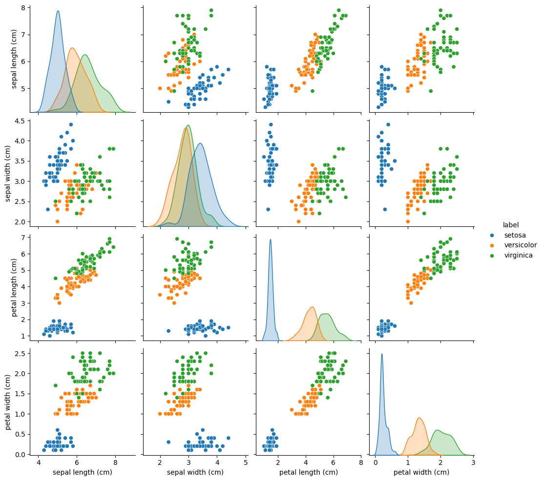
sns.pairplotを使えば、特徴を二つずつセットにして、散布図が作れます。
hueはクラスを指定します。
クラスに当たる列の名前を渡しましょう。
sns.pairplot(df2, hue="label")
<seaborn.axisgrid.PairGrid at 0x13ecbb110>
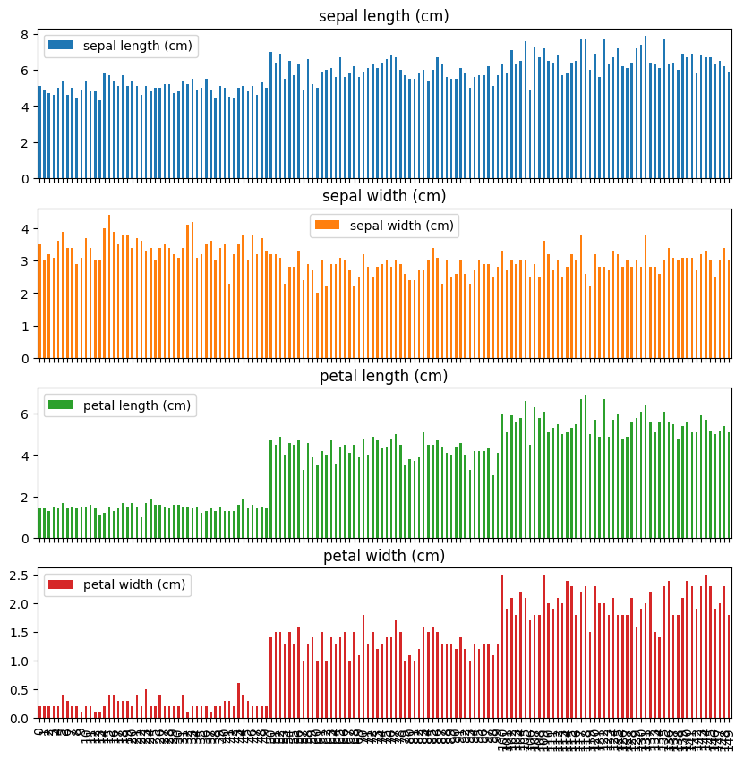
df.plotによる可視化#
df.plotメソッドで簡単にプロットができます。
seabornは統計学に特化した可視化ツールですが、plotメソッドでも一般的な可視化ができます。
kind引数に作りたいグラフの名前を入れてあげればOKです。
ちなみに引数がない場合は曲線になります。
df2.plot(
    kind="bar",      # グラフの種類
    subplots=True,   # subplotsをTrueにすると、列ごとに別のグラフを作れます。この引数を書かなければ一つにまとめられます。
    figsize=(10,10)  # figsizeでプロットサイズを指定できます。この引数を書かなくても適当なサイズで表示されます。
)
array([<Axes: title={'center': 'sepal length (cm)'}>,
       <Axes: title={'center': 'sepal width (cm)'}>,
       <Axes: title={'center': 'petal length (cm)'}>,
       <Axes: title={'center': 'petal width (cm)'}>], dtype=object)
統計量を計算#
要約統計量#
df2.describe()
| sepal length (cm) | sepal width (cm) | petal length (cm) | petal width (cm) | |
|---|---|---|---|---|
| count | 150.000000 | 150.000000 | 150.000000 | 150.000000 |
| mean | 5.843333 | 3.057333 | 3.758000 | 1.199333 |
| std | 0.828066 | 0.435866 | 1.765298 | 0.762238 |
| min | 4.300000 | 2.000000 | 1.000000 | 0.100000 |
| 25% | 5.100000 | 2.800000 | 1.600000 | 0.300000 |
| 50% | 5.800000 | 3.000000 | 4.350000 | 1.300000 |
| 75% | 6.400000 | 3.300000 | 5.100000 | 1.800000 |
| max | 7.900000 | 4.400000 | 6.900000 | 2.500000 |
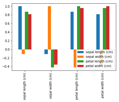
相関行列#
df2.corr()
---------------------------------------------------------------------------
ValueError                                Traceback (most recent call last)
Cell In[14], line 1
----> 1 df2.corr()

File ~/workspace/prpy/.venv/lib/python3.11/site-packages/pandas/core/frame.py:11049, in DataFrame.corr(self, method, min_periods, numeric_only)
  11047 cols = data.columns
  11048 idx = cols.copy()
> 11049 mat = data.to_numpy(dtype=float, na_value=np.nan, copy=False)
  11051 if method == "pearson":
  11052     correl = libalgos.nancorr(mat, minp=min_periods)

File ~/workspace/prpy/.venv/lib/python3.11/site-packages/pandas/core/frame.py:1993, in DataFrame.to_numpy(self, dtype, copy, na_value)
   1991 if dtype is not None:
   1992     dtype = np.dtype(dtype)
-> 1993 result = self._mgr.as_array(dtype=dtype, copy=copy, na_value=na_value)
   1994 if result.dtype is not dtype:
   1995     result = np.asarray(result, dtype=dtype)

File ~/workspace/prpy/.venv/lib/python3.11/site-packages/pandas/core/internals/managers.py:1694, in BlockManager.as_array(self, dtype, copy, na_value)
   1692         arr.flags.writeable = False
   1693 else:
-> 1694     arr = self._interleave(dtype=dtype, na_value=na_value)
   1695     # The underlying data was copied within _interleave, so no need
   1696     # to further copy if copy=True or setting na_value
   1698 if na_value is lib.no_default:

File ~/workspace/prpy/.venv/lib/python3.11/site-packages/pandas/core/internals/managers.py:1753, in BlockManager._interleave(self, dtype, na_value)
   1751     else:
   1752         arr = blk.get_values(dtype)
-> 1753     result[rl.indexer] = arr
   1754     itemmask[rl.indexer] = 1
   1756 if not itemmask.all():

ValueError: could not convert string to float: 'setosa'
df2.corr().plot(kind="bar")
<matplotlib.axes._subplots.AxesSubplot at 0x24d4bf4a5f8>
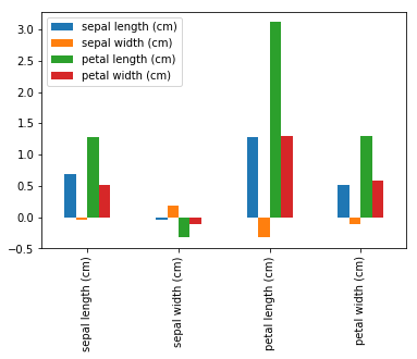
共分散行列#
df2.cov()
| sepal length (cm) | sepal width (cm) | petal length (cm) | petal width (cm) | |
|---|---|---|---|---|
| sepal length (cm) | 0.685694 | -0.039268 | 1.273682 | 0.516904 |
| sepal width (cm) | -0.039268 | 0.188004 | -0.321713 | -0.117981 |
| petal length (cm) | 1.273682 | -0.321713 | 3.113179 | 1.296387 |
| petal width (cm) | 0.516904 | -0.117981 | 1.296387 | 0.582414 |
df2.cov().plot(kind="bar")
<matplotlib.axes._subplots.AxesSubplot at 0x24d4d891518>